Quick start

import rectanglepy as rectangle
import pandas as pd
from anndata import AnnData, read_h5ad

Creating the input data

The tutorial data set contains single-cell RNA-seq counts as a pandas DataFrame, with the cell type annotations as a pandas Series.

The scRNA-seq data must come in the form of unnormalized gene counts, together with the associated cell-type annotations for the cell types of interest. The bulk RNA-seq data should be normalized as transcripts per million (TPM) –or counts per millions (CPM) in case of tag-based spatial transcriptomics. The gene nomenclature used for the single-cell and bulk datasets must match (e.g., gene synonyms) to provide meaningful results.

To see an example dataset, we can load the (small) tutorial data provided by Rectangle:

sc_counts, annotations, bulks  = rectangle.load_tutorial_data()

The tutorial data set contains (scRNA-seq data counts as a pandas DataFrame (cell by genes), with the cell-type annotations as a pandas Series (cell-type label for every cell ID).

sc_counts[['FCGR3A', 'RPL5', 'SF3B4','S100A10', 'ZBTB7B']].head()

	FCGR3A	RPL5	SF3B4	S100A10	ZBTB7B
E2L4_GATGCTACAGGCACAA	37	23	0	10	0
L5_AACAACCAGGAACTAT	0	15	0	12	2
L5_TCCTTCTGTACTCCGG	0	5	0	1	0
L2_GCCCGAACACGTATAC	0	15	1	12	1
E2L2_ATGCATGTCACACCCT	0	24	1	18	3

annotations.head()

E2L4_GATGCTACAGGCACAA    Monocytes
L5_AACAACCAGGAACTAT      Monocytes
L5_TCCTTCTGTACTCCGG      Monocytes
L2_GCCCGAACACGTATAC      Monocytes
E2L2_ATGCATGTCACACCCT    Monocytes
Name: 0, dtype: object

And the bulk RNA-seq data as a pandas DataFrame, where the index is the sample ID and the columns are the genes.

bulks[['FCGR3A', 'RPL5', 'SF3B4','S100A10', 'ZBTB7B']].head()

	FCGR3A	RPL5	SF3B4	S100A10	ZBTB7B
pbmc_1	145.144880	2505.165434	78.708398	415.135	49.318210
pbmc_10	137.999249	2296.208027	79.041928	475.642	53.047700
pbmc_12	456.966440	2544.939500	74.853167	443.532	45.043961

The count dataframe with its annotations can be easily convert into an AnnData object.

sc_adata = AnnData(sc_counts, obs=annotations.to_frame(name="cell_type"))

Single-step deconvolution

To deconvolute the bulk data in a single step, use the “rectangle()” function. This method returns the results of the signature-building step (signature_result) and a tuple with the estimated cell type proportions for every sample of the deconvolved bulk dataset (estimations)

estimations, signature_result = rectangle.rectangle(sc_adata, bulks)

The rectangle method returns two objects:

1. estimations: a pandas DataFrame with the estimated cell type proportions for each bulk sample.

2. signature_result: a RectangleSignatureResult object containing additional information about the signature and the unknown content.

#subset for better visualisation in the documentation
estimations.iloc[:, -5:]

	T cells CD8	Tregs	mDC	pDC	Unknown
pbmc_1	0.161062	0.426049	0.029880	0.002178	0.000000
pbmc_10	0.118129	0.392704	0.024096	0.004327	0.000000
pbmc_12	0.274570	0.255928	0.014791	0.003015	0.017726

signature_result

RectangleSignatureResult
──────────────────────────────────────────────────
  Total Signature genes: 143
  Cell types: 11
    B cells marker genes: ['ADAM28', 'BLK', 'CD22', 'CD37', 'CD79A', 'FCER2', 'FCRL1', 'HVCN1', 'P2RX5', 'PLPP5', 'RALGPS2', 'SNX2', 'STRBP', 'VPREB3', 'ZCCHC7']
    ILC marker genes: ['C16orf54', 'CD7', 'HTATSF1', 'IL18R1']
    Monocytes marker genes: ['ADAP2', 'AGTRAP', 'ALDH3B1', 'ATG16L2', 'BCL6', 'BEST1', 'BST1', 'CAMKK2', 'CD300E', 'CD300LF', 'CD302', 'CEBPB', 'CFD', 'CLEC12A', 'CLEC7A', 'CPPED1', 'CREG1', 'CSF3R', 'DUSP1', 'DUSP6', 'EMILIN2']
    NK cells marker genes: ['C1orf21', 'CEP78', 'CST7', 'CTBP2', 'CX3CR1', 'FCGR3A', 'FGFBP2', 'GNLY', 'GNPTAB', 'GZMH', 'IL2RB', 'ITGAL', 'KLRC1', 'MYBL1', 'SAMD3', 'SPON2', 'SYNE1', 'TBX21']
    Plasma cells marker genes: ['ARSA', 'ATP13A1', 'CALR', 'CDK14', 'CKAP4', 'COPB2', 'DEF8', 'EIF2AK3', 'ERLEC1', 'FAM136A', 'FAM3C', 'FKBP2', 'FNDC3B', 'GMPPA', 'GORASP2', 'HIBCH', 'HM13', 'LAX1', 'MAN1A1', 'MANF', 'MLEC']
    Platelet marker genes: ['ACRBP', 'CCL5', 'CMTM5', 'CTDSPL', 'DAB2', 'DAPP1', 'FERMT3', 'GRAP2', 'ILK', 'KIF2A', 'LEPROT', 'MAP3K7CL', 'MAX', 'MGAT4B', 'MMD', 'MPP1', 'MTURN', 'OAZ1', 'PF4', 'PGRMC1', 'PRKAR2B']
    T cells CD4 conv marker genes: ['MAL']
    T cells CD8 marker genes: ['CD8A']
    Tregs marker genes: ['MAL']
    mDC marker genes: ['ANXA2', 'ATP1B1', 'BATF3', 'CACNA2D3', 'CIITA', 'EMILIN2', 'FCGR2B', 'FCGRT', 'GPAT3', 'GRASP', 'HLA-DPB1', 'HLA-DQB1', 'HLA-DRB5', 'IGSF6', 'IL13RA1', 'IL18', 'JAML', 'LGALS1', 'LGALS2', 'PAK1', 'RAB34']
    pDC marker genes: ['AEBP1', 'ARHGAP27', 'ASIP', 'ATG101', 'BCL7A', 'C12orf75', 'CBX4', 'CCDC186', 'CHML', 'CLN8', 'CRYBG3', 'CUEDC1', 'CXorf21', 'CYP46A1', 'EIF4A3', 'EPHB1', 'FAM129C', 'FLT3', 'FMNL3', 'GAS6', 'GPM6B']
  Cluster assignments: ['B cells', 'ILC', 6, 2, 'Plasma cells', 'Platelet', 1, 2, 1, 6, 'pDC']
  Unknown cell content analysis: Yes
  DGE Optimization result available:
    Best cutoffs: p: 0.05, lfc: 1.6

2-step deconvolution

Rectangle can also be run in two steps, first creating the signature and then deconvolving the bulk data.

1. Create Signature result

signature_result = rectangle.pp.build_rectangle_signatures(sc_adata, bulks=bulks)

This creates a RectangleSignatureResult object.

2. Deconvolve bulk data

We can then use the signature result to deconvolve the bulk data. This is done using the deconvolution method of the RectangleSignatureResult object, which should be fed with the signature_result object obtained at the previous step and the bulk dataset to be deconvolved

estimations, _ = rectangle.tl.deconvolution(signature_result, bulks)

This call returns a pandas DataFrame with the estimated cell type proportions.

#subset for better visualisation in the documentation
estimations.iloc[:, -5:]

	T cells CD8	Tregs	mDC	pDC	Unknown
pbmc_1	0.161062	0.426049	0.029880	0.002178	0.000000
pbmc_10	0.118129	0.392704	0.024096	0.004327	0.000000
pbmc_12	0.274570	0.255928	0.014791	0.003015	0.017726

Bulk RNA-seq deconvolution

To apply Rectangle to a more meaningful use case, we will perform the deconvolution of 9 bulk RNA-seq samples from blood-cell mixtures generated in the [FMP+19] study. We can access this dataset from deconvData[DMP+24]

url = "https://figshare.com/ndownloader/files/44877523"
bulks_fino = pd.read_csv(url, index_col=0)
bulks_fino.T[['LYZ', 'CD14', 'FCGR3A', 'CD8A', 'CD3D']].head()

	LYZ	CD14	FCGR3A	CD8A	CD3D
pbmc_1	7912.41	645.8500	145.144880	123.580148	357.85446
pbmc_10	9331.48	800.9088	137.999249	99.817693	258.58275
pbmc_12	9506.39	512.9779	456.966440	179.161160	328.40886
pbmc_2	6048.82	505.6502	158.455478	87.202916	320.96350
pbmc_4	3547.27	288.5666	314.124590	175.999580	267.81102

To train rectangle and build the signature matrix, we will use single-cell dataset human peripheral blood mononuclear cells (PBMC) profiled with the CITE-seq technology in the Hao et al. study [HHAN+21]. We will use a reduced and reannotated version of this dataset which is accessible through deconvData

# the files are originaly in an rds format,
# we skip the conversion step here and load an AnnData object directly
haoSub_adata = read_h5ad("../data/haoSub_adata.h5ad")
haoSub_adata

AnnData object with n_obs × n_vars = 14744 × 24049
    obs: 'cell_type'

We can now use the rectangle method to deconvolute the bulk data guided by the single-cell expression profiles and annotations using just a single command.

estimations, signature_result = rectangle.rectangle(haoSub_adata, bulks_fino.T)

The estimated cell-type fractions can be visualized in Python as a stacked barplot using matplotlib:

import matplotlib.pyplot as plt

fig, ax = plt.subplots(dpi=200)  # Increased resolution
colors = plt.get_cmap('tab20').colors  # More distinct colors
estimations.plot(kind='bar', stacked=True, ax=ax, color=colors)
ax.set_title('Rectangle deconvolution Results (Finotello dataset)', fontsize=16)
ax.set_ylabel('Cell fractions (%)', fontsize=14)
ax.set_xlabel('Bulk sample', fontsize=14)
ax.legend(title='Cell type', bbox_to_anchor=(1.05, 1), loc='upper left', fontsize=12)
plt.tight_layout()
plt.show()

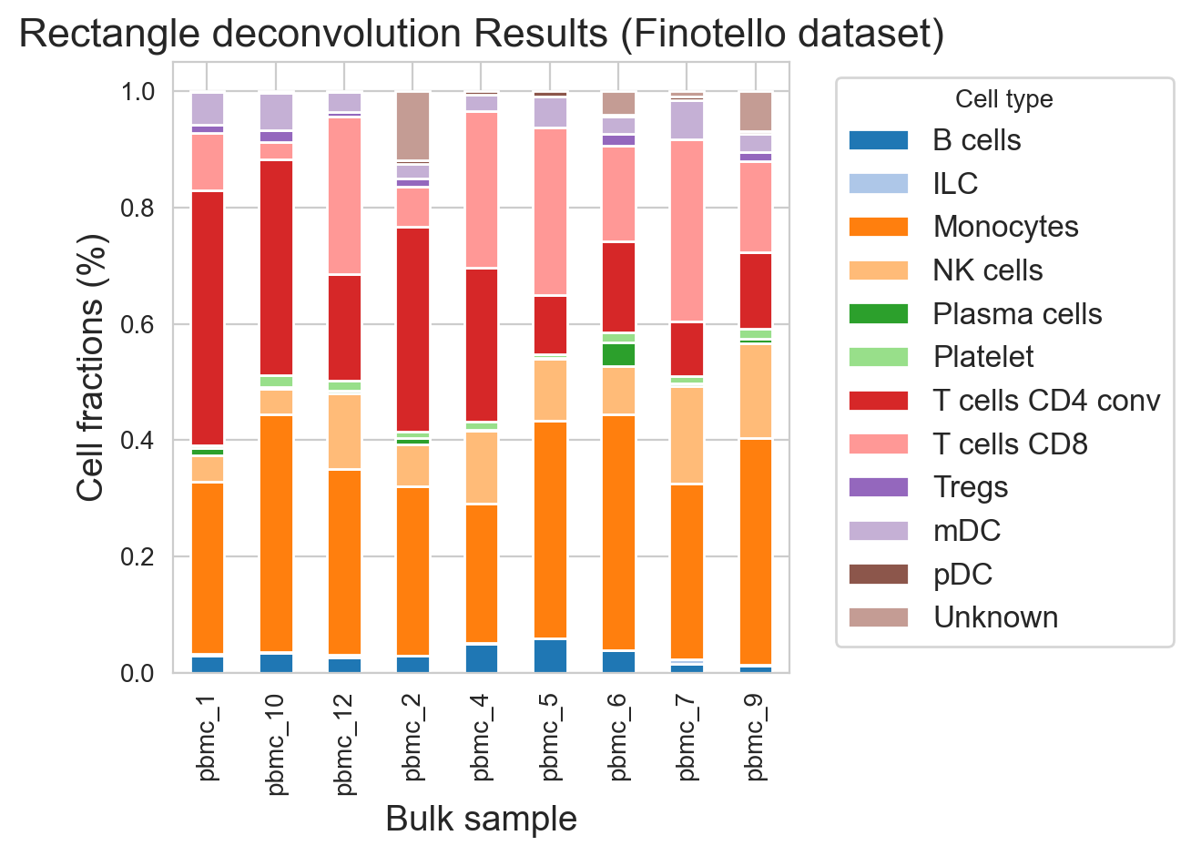
The Finotello dataset also provides ground-truth cell fractions obtained via fluorescence-activated cell sorting (FACS) from all the analyzed bulk samples, which can be used to validate Rectangle estimates.

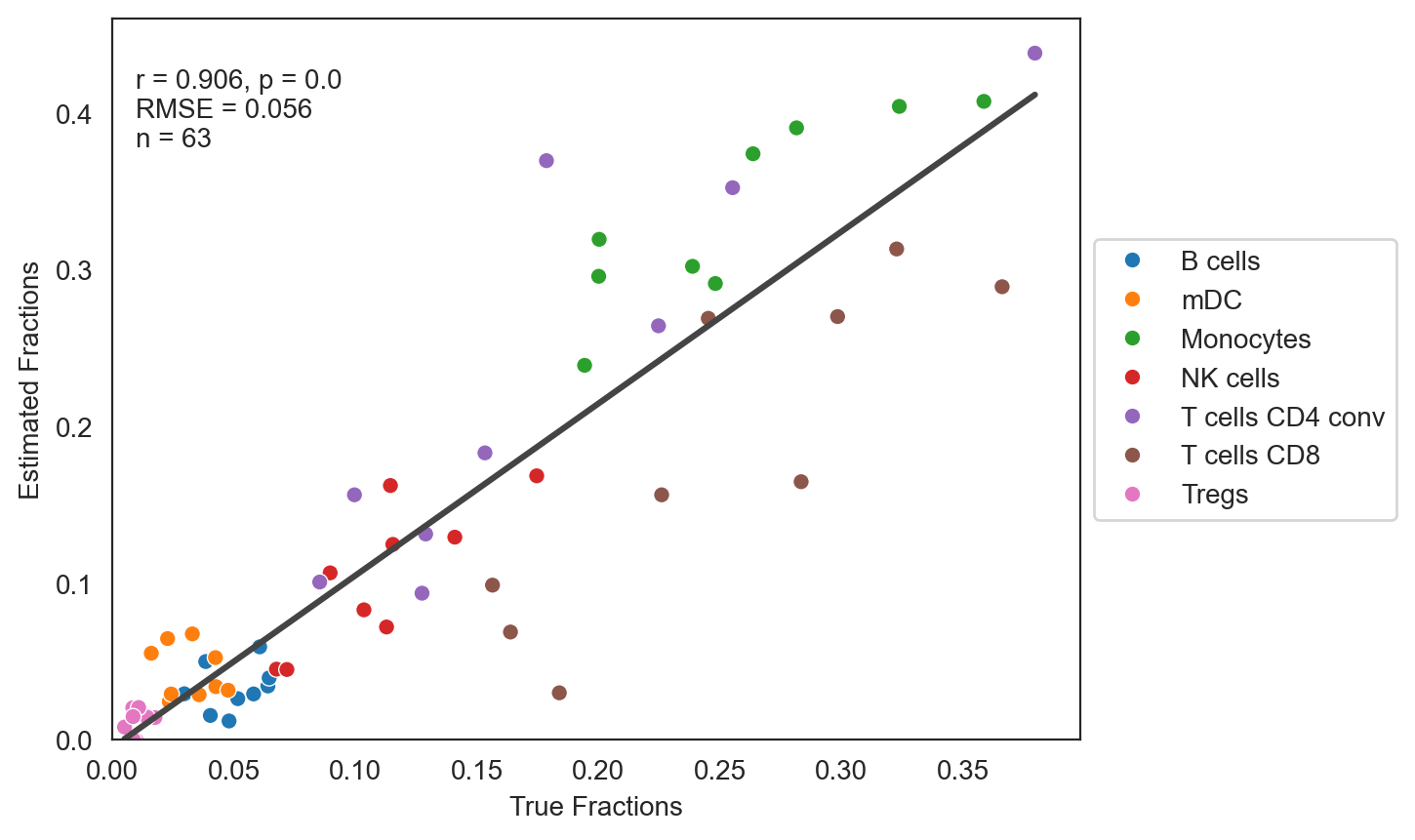
So let us further explore the estimation performance by plotting the estimated cell type proportions against the true cell type proportions we can again obtain from deconvData.

url = "https://figshare.com/ndownloader/files/44877526"
finotello_true = pd.read_csv(url, index_col=0).T
# rename the columns to match the cell types in the estimations
finotello_true.columns = ["NK cells", 'B cells', 'Tregs', 'mDC', 'Monocytes', 'Neutrophils', 'T cells CD8',
                         'T cells CD4 conv', 'Other']

First, we need to do some data wrangling to make the data compatible.

# funtion to match the dataframes by index and columns
# and sort them by index and columns
def match_dfs(df1, df2):
    common_rows = df1.index.intersection(df2.index)
    common_cols = df1.columns.intersection(df2.columns)
    df1_matched = df1.loc[common_rows, common_cols].sort_index().sort_index(axis=1)
    df2_matched = df2.loc[common_rows, common_cols].sort_index().sort_index(axis=1)
    return df1_matched, df2_matched

# function to create a dataframe for evaluation
# it takes the expected and estimated dataframes and returns a melted dataframe
def create_evaluation_df(expected_df, estimated_df):
    evaluation_df = expected_df.T.melt()
    estimated_df_e = estimated_df.T.melt()
    evaluation_df['result'] = estimated_df_e['value']
    evaluation_df.columns = ['Cell type','True Fractions' , 'Estimated Fractions']
    return evaluation_df

true_m, finotello_m = match_dfs(finotello_true.T, estimations.T)
true_m = true_m.sort_index(key=lambda x: x.str.lower())
finotello_m = finotello_m.sort_index(key=lambda x: x.str.lower())

evaluation_df = create_evaluation_df(true_m, finotello_m)

Next, we quantitatively compare Rectangle estimates to the ground-truth cell fractions using Pearson correlation (r) and root-mean square error (RMSE), as well as cell-fraction scatter plots:

import numpy as np
from scipy.stats import pearsonr
import seaborn as sns

def evaulate_total_df(df):
    rsme_total = np.sqrt(np.mean((df['Estimated Fractions'] - df['True Fractions']) ** 2))
    r_value_total, p_value_total =  pearsonr(df['Estimated Fractions'], df['True Fractions'])
    return rsme_total, r_value_total, p_value_total

rsme_finotello_rectangle, r_finotello_rectangle, p_finotello_rectangle = evaulate_total_df(evaluation_df)

def create_scatter_plot_total(df, rsme, p_value, r_value, title="Total", y_axis_label="Estimated Fractions", x_axis_label="True Fractions", hue="Cell type"):
    sns.set_style("white")
    fig, ax = plt.subplots(dpi=200)  # Increased resolution
    g = sns.scatterplot(x="True Fractions", y="Estimated Fractions",hue=hue, data=df, ax=ax)
    sns.regplot(x="True Fractions", y="Estimated Fractions", data=df, scatter=False, color='#444444', ci=None, ax=ax)
    text = f"r = {round(r_value, 3)}, p = {round(p_value, 10)} \nRMSE = {round(rsme, 3)}\nn = {len(df)}"
    g.set(xlabel=x_axis_label, ylabel=y_axis_label)
    g.legend(loc='center left', bbox_to_anchor=(1, 0.5))
    g.annotate(text, xy=(0.01, 0.95), xycoords="axes fraction",
                xytext=(5, -5), textcoords="offset points",
                ha="left", va="top")
    g.set_xlim(0, g.get_xlim()[1])
    g.set_ylim(0, g.get_ylim()[1])
    return g

rsme_finotello_rectangle, r_finotello_rectangle, p_finotello_rectangle = evaulate_total_df(evaluation_df)
create_scatter_plot_total(evaluation_df, rsme_finotello_rectangle, p_finotello_rectangle, r_finotello_rectangle)

<Axes: xlabel='True Fractions', ylabel='Estimated Fractions'>

Spatial deconvolution

Rectangle can be also effectively applied to spot-based spatial transcriptomics data, seamlessly integrating with the spatialdata package. See the spatialdata documentation for more details.

The mouse brain slide “ST8059048” was downloaded from ArrayExpress, with access number E-MTAB-11114 [HYH+22]. Find the dataset in https://figshare.com/articles/dataset/Tutorial_data/30104548?file=58967194

import spatialdata_io
import pandas as pd
import numpy as np
from anndata import AnnData, read_h5ad

s_data = spatialdata_io.visium(path='../data/spatial_ST8059048', dataset_id='ST8059048', scalefactors_file='scalefactors_json.json', tissue_positions_file='tissue_positions_list.csv', counts_file='ST8059048_filtered_feature_bc_matrix.h5')

Single-cell data: scRNA-seq data from the mouse brain was downloaded from Array Express, with accession number E-MTAB-11115 [KSD+22]. You can find a description of the preprocessing steps in https://figshare.com/articles/dataset/Tutorial_data/30104548?file=58978408

Find the processed data in https://figshare.com/articles/dataset/Tutorial_data/30104548?file=58978435

adata = read_h5ad('../data/cell2location_single_cell_processed.h5ad')

We can run Rectangle on the spatial data using the rectangle method, by using the ‘table’ object of the SpatialData object. As the spatial expression data is summarized as raw gene counts, we will first convert it to CPM.

data_table = s_data['table']
bulks = data_table.to_df()
bulks_cpm = bulks.div(bulks.sum(axis=1), axis=0) * 1e6

estimations, signature_result = rectangle.rectangle(adata, bulks_cpm)

# remove disconnected spots
disconnected_spots = ["AATCGAGGTCTCAAGG-1", "ACCACACGGTTGATGG-1",
                   "ACCGAGTCTCCTTATT-1", "AGCAGTCGAAGCATGC-1",
                   "AGTACAGAAGCTTATA-1", "CCTACAGTTGAGGGAG-1",
                   "CGCTTTCCGCCAAGGT-1", "CGGTATGGGCACTCTG-1",
                   "CGGTTGGGCAGGGTCC-1", "CTATCACAACGCTGGA-1",
                   "CTCTAACACCGGCAGC-1", "CTTACATAGATTTCTT-1",
                   "CTTCATCACCAGGGCT-1", "GAAGGGTCATTAAGAC-1",
                   "GACCACACTTCCCTTT-1", "GCACGCCGATTCCCGC-1",
                   "GCGGCTTTAGCAAGTT-1", "GCGTCGTAACATGGTC-1",
                   "GGATTAATCATGGACC-1", "GTACTACGGCCTCGTT-1",
                   "TACACAGCCGTGGTGC-1", "TCAGCGCACGCCGTTT-1",
                   "TGCCCGATAGTTAGAA-1", "TGTAGCCAATTCCGTT-1"]
estimations = estimations.drop(index=disconnected_spots)

We can add our estimations to the spatial data by creating a new AnnData object from the estimations and adding it to the SpatialData object.

from spatialdata.models import TableModel

# Create AnnData from estimations
table_data = AnnData(estimations)

# Add the required metadata columns
table_data.obs['region'] = 'ST8059048'
table_data.obs['instance_id'] = table_data.obs.index

adata_for_sdata = TableModel.parse(
    table_data,
    region='ST8059048',
    region_key='region',
    instance_key='instance_id'
)

s_data.tables["rectangle_results"] = adata_for_sdata